```python
# Import libraries
import warnings
import pandas as pd
import psutil
import sklearn
from statsmodels.tsa.seasonal import seasonal_decompose
import numpy as np
import seaborn as sns
import matplotlib.pyplot as plt
from sklearn.neural_network import MLPRegressor
from sklearn.neighbors import KNeighborsRegressor
from sklearn.svm import SVR
from sklearn.ensemble import RandomForestRegressor
from sklearn.tree import DecisionTreeRegressor
from sklearn.linear_model import LinearRegression
from sklearn.metrics import mean_squared_error, mean_absolute_error, r2_score
```
# Data Preprocessing
```python
# Load the dataset
df = pd.read_csv('data/monthly-sunspots.csv')
df.head()
```
|
Month |
Sunspots |
| 0 |
1749-01 |
58.0 |
| 1 |
1749-02 |
62.6 |
| 2 |
1749-03 |
70.0 |
| 3 |
1749-04 |
55.7 |
| 4 |
1749-05 |
85.0 |
```python
df.shape
```
(2820, 2)
```python
# convert the date column to datetime
df['Month'] = pd.to_datetime(df['Month'], format='%Y-%m')
df.head()
```
|
Month |
Sunspots |
| 0 |
1749-01-01 |
58.0 |
| 1 |
1749-02-01 |
62.6 |
| 2 |
1749-03-01 |
70.0 |
| 3 |
1749-04-01 |
55.7 |
| 4 |
1749-05-01 |
85.0 |
```python
df.tail()
```
|
Month |
Sunspots |
| 2815 |
1983-08-01 |
71.8 |
| 2816 |
1983-09-01 |
50.3 |
| 2817 |
1983-10-01 |
55.8 |
| 2818 |
1983-11-01 |
33.3 |
| 2819 |
1983-12-01 |
33.4 |
```python
df.sort_values(by='Month', inplace=False).tail()
```
|
Month |
Sunspots |
| 2815 |
1983-08-01 |
71.8 |
| 2816 |
1983-09-01 |
50.3 |
| 2817 |
1983-10-01 |
55.8 |
| 2818 |
1983-11-01 |
33.3 |
| 2819 |
1983-12-01 |
33.4 |
```python
df.Sunspots.sum()
```
144570.0
```python
# sum by years
df_grouped = df.groupby(pd.Grouper(key='Month', freq='Y')).sum()
df_grouped.head()
```
|
Sunspots |
| Month |
|
| 1749-12-31 |
971.1 |
| 1750-12-31 |
1000.7 |
| 1751-12-31 |
571.9 |
| 1752-12-31 |
573.6 |
| 1753-12-31 |
368.3 |
```python
# set the date column as the index
df_indexed = df.set_index('Month', inplace=False)
```
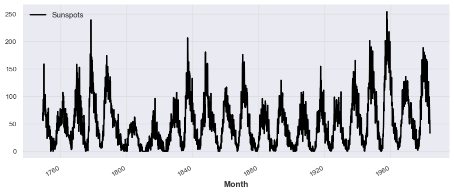
The data is already ordered by date. The first date is 1749-01-01 and the last is 1983-12-01. The sample is a month with its number of Sunspots registered. The data is a time series.
The sunspot number is a float, this means that is either an average or it keeps track of partial sunspots that end/start in a different month. Probably the latter since the total number of sunspots is an integer. But we can't be sure. This shouldn't matter for our model training anyway. Also, the total number is even probably because the sunspots appears in pairs. This could be useful for our model.
_Sunspots are temporary phenomena on the Sun's photosphere that appear as spots darker than the surrounding areas. They are regions of reduced surface temperature caused by concentrations of magnetic field flux that inhibit convection. Sunspots usually appear in pairs of opposite magnetic polarity. Their number varies according to the approximately 11-year solar cycle._
_The sunspot number is a crucial component of space weather. It is a measure of solar activity, and the number of sunspots on the solar surface changes over the course of the solar cycle. The solar cycle is a periodic change in the sun's activity and appearance. The cycle is about 11 years long on average. The solar cycle is marked by the increase and decrease of sunspots on the sun's surface. During the solar maximum, large numbers of sunspots appear, and during the solar minimum, very few sunspots appear. The solar cycle affects space weather, which can affect satellites and astronauts in space. The solar cycle is also responsible for the aurora borealis, or Northern Lights, in the Northern Hemisphere. The solar cycle was discovered in 1843 by Samuel Heinrich Schwabe, who noticed that the number of sunspots visible on the sun's surface changed over time. The solar cycle is also known as the sunspot cycle or the Schwabe cycle._
```python
df_indexed.describe()
```
|
Sunspots |
| count |
2820.000000 |
| mean |
51.265957 |
| std |
43.448971 |
| min |
0.000000 |
| 25% |
15.700000 |
| 50% |
42.000000 |
| 75% |
74.925000 |
| max |
253.800000 |
The
```python
df_indexed.info()
```
DatetimeIndex: 2820 entries, 1749-01-01 to 1983-12-01
Data columns (total 1 columns):
# Column Non-Null Count Dtype
--- ------ -------------- -----
0 Sunspots 2820 non-null float64
dtypes: float64(1)
memory usage: 44.1 KB
THere is no missing values in the dataset.
```python
# print a boxplot
sns.boxplot(x=df_indexed['Sunspots'])
```
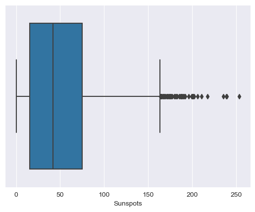
Also, no extreme values are present.
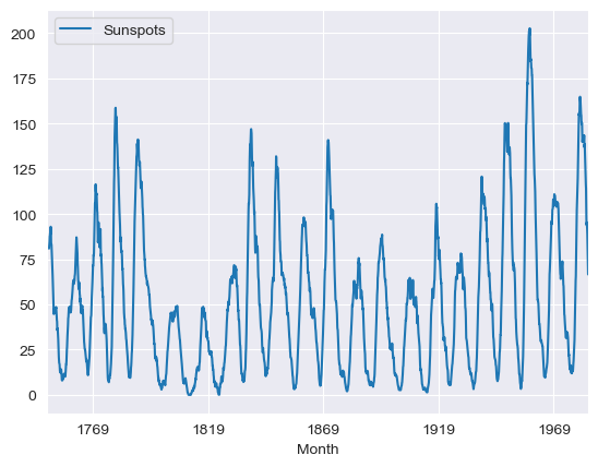
# Data Visualization
Since the data is a time series, we can plot the data to see how the sunspots have changed over time. I will use the seaborn library to plot the data. Since the result is better than matplotlib.
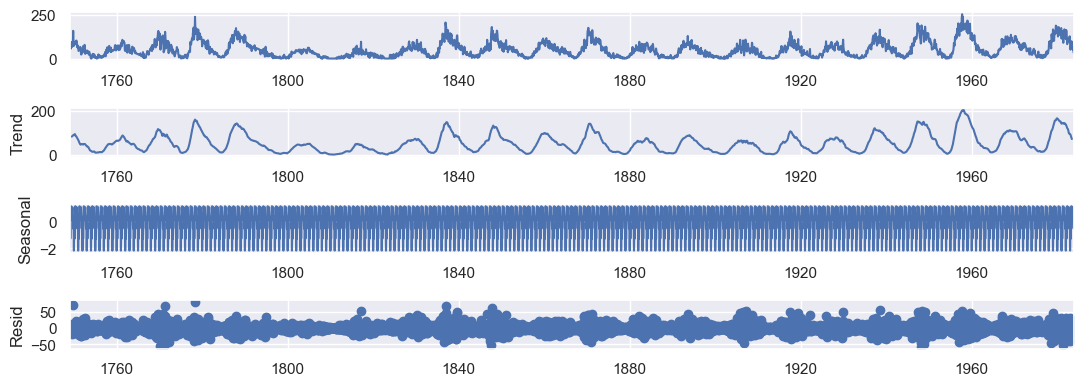
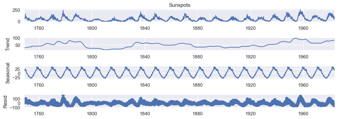
- Trend Component: It represents the long-term pattern or trend in the data. It shows the overall direction or tendency of the data over an extended period. The trend component indicates whether the series is increasing, decreasing, or remaining relatively stable.
- Seasonal Component: It represents the repetitive pattern or seasonality in the data. It captures the periodic fluctuations that occur over a specific time period, such as daily, weekly, or yearly patterns.
- Residual Component: It represents the remaining or leftover variation in the data after removing the seasonal and trend components. It consists of the random fluctuations, noise, or irregularities that cannot be explained by the seasonal or trend patterns.
```python
# get rolling mean on a year basis
rolling_mean = df_indexed.rolling(window=12).mean().plot()
```
```python
result = seasonal_decompose(df_indexed, model='additive')
sns.set(rc={'figure.figsize':(11, 4)})
ax = result.plot()
```
```python
# same but in a shorted range
df_short = df_indexed['1820-01-01':'1870-01-01']
result = seasonal_decompose(df_short, model='additive')
sns.set(rc={'figure.figsize':(11, 4)})
ax = result.plot()
```
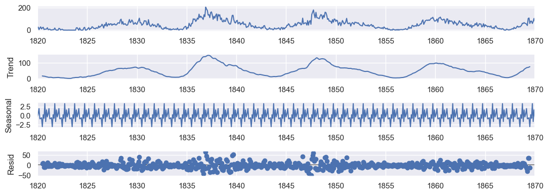
We can see a *trend* which start at 0 sunspots and increase to some number of sunspots. Then it decrease to 0 sunspots again. Graphically, this is a cycle seems to be around 10 years. We know that it is 11 years.
The *seasonal* component has a variance between -2.5 and 2.5.
The *residual* component is the noise around the trend and seasonal component.
```python
# zooming a specific trend
df_trend = df_indexed['1832-01-01':'1844-01-01']
result = seasonal_decompose(df_trend, model='additive')
# plot with sns
sns.set(rc={'figure.figsize':(11, 4)})
ax = result.plot()
```
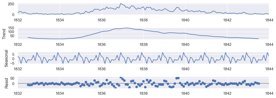
The residual component is the noise around the trend and seasonal component. It is vary between -50 and 50.
# Fourier Transform
Apply the Fourier transformation and find the periodicity of the data.
The Fourier transform is a mathematical function that takes a time-based pattern as input and determines the overall cycle offset, rotation speed, and strength for every possible cycle in the given pattern. The Fourier transform is used to find the cyclic patterns hidden in the time series data.
I will calculate the periodicity on the train set to avoid test bias.
```python
df_train = df_indexed['1749-01-01':'1919-12-01']
df_test = df_indexed['1920-01-01':'1983-12-01']
df_train.shape, df_test.shape
```
((2052, 1), (768, 1))
```python
# Apply Fourier transformation
fourier_transform = np.fft.fft(df_train['Sunspots'])
fourier_transform.shape
```
(2052,)
```python
fourier_transform[0:10]
```
array([93338.8 +0.j , 1468.1036331 -212.88095452j,
-1264.72141466-17793.04535383j, -7928.54620491 +6239.67068341j,
7122.83407343 +3535.55795089j, 555.94555365 +206.05242238j,
3791.90814354 -5119.83490291j, 1853.86932136 +4123.29141588j,
3675.5880518 +5597.02967995j, 963.21680018 -2620.91520629j])
```python
# Compute the frequencies corresponding to the Fourier coefficients
n = len(df_train['Sunspots'])
frequencies = np.fft.fftfreq(n)
frequencies.shape
```
(2052,)
```python
frequencies[0:10]
```
array([0. , 0.00048733, 0.00097466, 0.00146199, 0.00194932,
0.00243665, 0.00292398, 0.00341131, 0.00389864, 0.00438596])
```python
# Find the periodicity (frequency with the highest amplitude)
periodicity = np.abs(frequencies[np.argmax(np.abs(fourier_transform))])
print('Periodicity =', periodicity)
```
Periodicity = 0.0
```python
print(f"Periodicity: {1 / periodicity} time units")
```
Periodicity: inf time units
C:\Users\Administrator\AppData\Local\Temp\ipykernel_82340\2936873598.py:1: RuntimeWarning: divide by zero encountered in scalar divide
print(f"Periodicity: {1 / periodicity} time units")
A periodicity of "infinite" is not what we would expect.
```python
# Plot the Fourier transform
plt.figure(figsize=(12, 4))
plt.plot(frequencies, np.abs(fourier_transform))
plt.xlabel('Frequency')
plt.ylabel('Amplitude')
plt.xlim(0, 0.02)
plt.show()
```
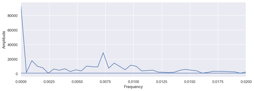
The code return a very high periodicity near 0. But this is wrong, the periodicity we want is the second peak we see. so I will recalculate the argmax but ignoring the first peak.
```python
# Find the periodicity (frequency with the highest amplitude)
threshold = 5
max_index = np.argmax(np.abs(fourier_transform[threshold:])) + threshold
periodicity = 1 / np.abs(frequencies[max_index])
print('Periodicity =', periodicity)
```
Periodicity = 136.8
This means a periodicity if 136.8 months. Which is 11.4 years. This is the expected periodicity of the sunspots.
For the future engineering, I will use the periodicity of 11.4 years.
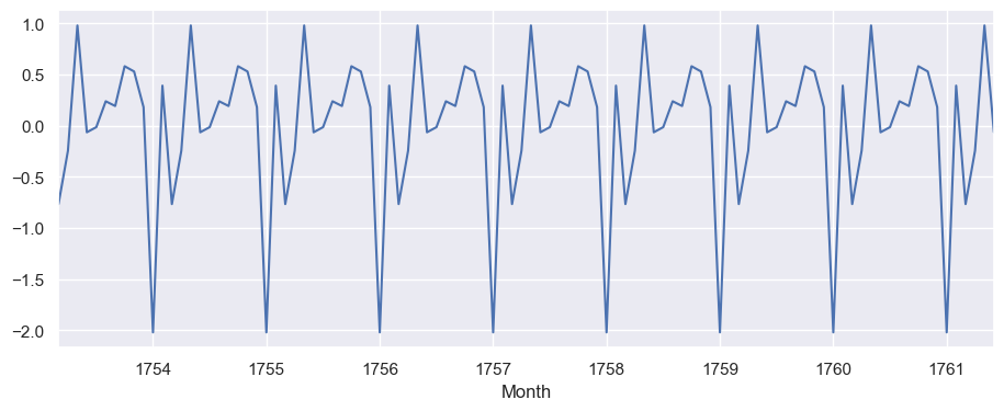
I will also calculate the periodicity of the seasonality.
```python
# Plot the Fourier transform but this time only for the seasonality
result_season = seasonal_decompose(df_train, model='additive').seasonal
result_season.iloc[50:150].plot()
```
```python
n_season = len(result_season)
frequencies_season = np.fft.fftfreq(n_season)
fourier_transform_season = np.fft.fft(result_season)
plt.figure(figsize=(12, 4))
plt.plot(frequencies_season, np.abs(fourier_transform_season))
plt.xlabel('Frequency')
plt.ylabel('Amplitude')
plt.xlim(0, 0.1)
plt.show()
```
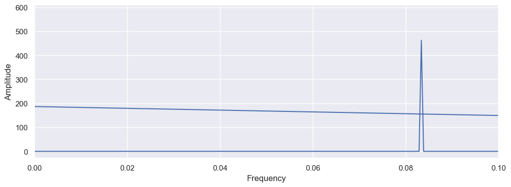
```python
threshold = 0
max_index_season = np.argmax(np.abs(fourier_transform_season[threshold:])) + threshold
frequencies_season[max_index_season]
```
0.3333333333333333
It returns 0.333, but its clearly wrong looking at the graph, so, as a feature, I will use the seasonality of 0.083 which is 12.1 months.
# Model Training
## Test and Train Split
Data before 1920 as train.
```python
# Split in the furrier transform section
df_train = df_indexed['1749-01-01':'1919-12-01']
df_test = df_indexed['1920-01-01':'1983-12-01']
df_test.head()
```
|
Sunspots |
| Month |
|
| 1920-01-01 |
51.1 |
| 1920-02-01 |
53.9 |
| 1920-03-01 |
70.2 |
| 1920-04-01 |
14.8 |
| 1920-05-01 |
33.3 |
## Baseline Model
As a baseline model, I will use the mean of the train data as the prediction for the test data.
### Mean of the Train Data
```python
# Create a baseline model
baseline_model = np.full(len(df_test), df_train['Sunspots'].mean())
baseline_model[0:10]
```
array([45.48674464, 45.48674464, 45.48674464, 45.48674464, 45.48674464,
45.48674464, 45.48674464, 45.48674464, 45.48674464, 45.48674464])
### Evaluation Metrics
I will use the following metrics to evaluate the model:
- RMSE (Root Mean Squared Error): It is the square root of the average of squared differences between prediction and actual observation. It measures the standard deviation of residuals.
- MAE (Mean Absolute Error): It is the average of the absolute differences between prediction and actual observation. It measures the average magnitude of errors in a set of predictions, without considering their direction.
- R2 (R-Squared): It is the proportion of the variance in the dependent variable that is predictable from the independent variable(s). It measures how close the data are to the fitted regression line. Nearest to 1 is better.
```python
# Calculate the RMSE (Root Mean Squared Error)
baseline_rmse = np.sqrt(mean_squared_error(df_test['Sunspots'], baseline_model))
print('Baseline RMSE:', baseline_rmse)
# Calculate the MAE (Mean Absolute Error)
baseline_mae = mean_absolute_error(df_test['Sunspots'], baseline_model)
print('Baseline MAE:', baseline_mae)
# Calculate the R2 score
baseline_r2 = r2_score(df_test['Sunspots'], baseline_model)
print('Baseline R2:', baseline_r2)
```
Baseline RMSE: 56.73590776250707
Baseline MAE: 43.43141345841456
Baseline R2: -0.16264654387789323
```python
# Plot the baseline model
plt.figure(figsize=(12, 4))
plt.plot(df_train.index, df_train['Sunspots'], label='Train')
plt.plot(df_test.index, df_test['Sunspots'], label='Test')
plt.plot(df_test.index, baseline_model, label='Baseline model')
plt.legend(loc='upper left')
mae = mean_absolute_error(df_test, baseline_model)
mse = mean_squared_error(df_test, baseline_model)
r2 = r2_score(df_test, baseline_model)
plt.title(f"Model: Baseline", fontsize=16, fontweight='bold')
plt.text(0.5, 0.9, f"MAE: {mae:.2f}", transform=plt.gca().transAxes)
plt.text(0.5, 0.85, f"MSE: {mse:.2f}", transform=plt.gca().transAxes)
plt.text(0.5, 0.8, f"R^2: {r2:.2f}", transform=plt.gca().transAxes)
```
Text(0.5, 0.8, 'R^2: -0.16')
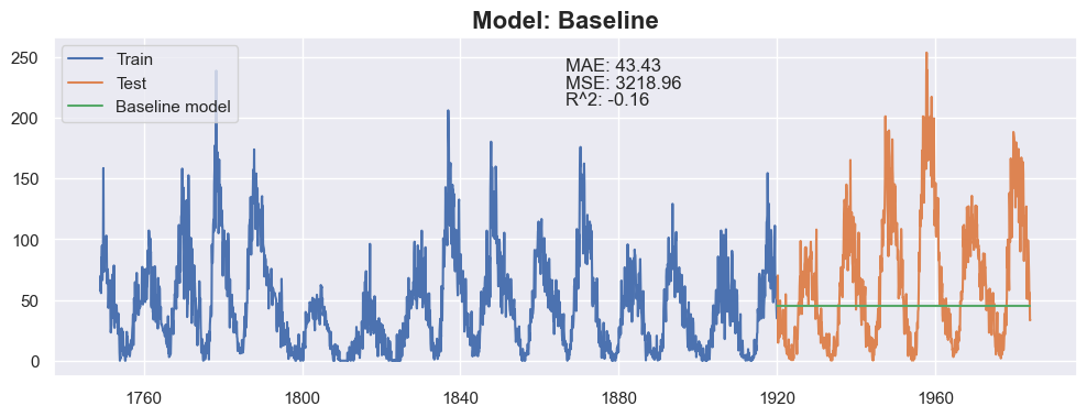
This clearly doesn't look good. Let's see if we can do better.
## Train and Compare Models
I will create the features to train the model, the month and the year.
### Features Engineering
Since the date itself is a bad feature, I need to create them, to train the model:
- The month: a number between 1 and 12 that indicates the month of the year.
- The partial: a number between 0 and 133 that indicate the month of the cycle. The cycle is 134.29 months long, so the partial is the number of months since the last cycle.
- The trend: the trend is the long-term increase or decrease in the data. It is the overall pattern of the data. It is the trend that the model will try to predict.
- The noise: the noise is the difference between the actual observation and the prediction of the previous model. It is the noise around the trend and seasonal component.
- The seasonality: the seasonality is the periodic component of the data. It is the repeating pattern within each year.
```python
plt_seasonal_dec = seasonal_decompose(df_indexed['Sunspots'], model='additive', period=134, extrapolate_trend='freq', two_sided=True).plot()
```
```python
df_train = df_indexed['1749-01-01':'1919-12-01']
df_test = df_indexed['1920-01-01':'1983-12-01']
def parse_df(df_: pd.DataFrame, trend_period: int = 137, seasonal_period: int = 12, window_size: int = 3) -> pd.DataFrame:
df_ret = pd.DataFrame(columns=[#'Month-total', # The month number since the beginning of the data (preserve total time information)
# 'Partial-trend-month', # The month number since the beginning of the cycle
# 'Partial-seasonal-month', # The month number since the beginning of the seasonality
# 'rolling-avg-3', # The rolling average, gives information about the sunspots numbers
# 'rolling_change', # The rolling difference, gives information about the direction
# 'Trend',
# 'Noise',
# 'Seasonality'
])
# df_ret['Month-total'] = df_.index.month + (df_.index.year - 1749) * 12
df_ret['Partial-trend-month'] = ((df_.index.year - 1749) * 12 + df_.index.month) % trend_period
df_ret['Partial-seasonal-month'] = ((df_.index.year - 1749) * 12 + df_.index.month) % seasonal_period
rolling_avg = df_['Sunspots'].rolling(window=3, min_periods=1).mean().to_frame()['Sunspots']
rolling_diff = df_['Sunspots'].diff(periods=1).to_frame()['Sunspots']
rolling_diff.fillna(0, inplace=True)
df_ret.index = df_.index
# to add the information about the speed of the change
# I wanted to get the rolling derivative or the gradient, but there is no function for that, however,
# I found out the percentage change function (only version 2.0.1+)
# which gives the percentage change between the current and a prior element(s). (it doesn't work)
# rolling_change = df_['Sunspots'].pcnt_change(window_size)
# I will calculate simply by doing: Dy/Dx where x is the time and y is the sunspots
# print i will use 3 month as the time step
# rolling sum of the last 3 months
rolling_der = df_['Sunspots'].diff(periods=1).to_frame()['Sunspots']
# fill the first 2 values with the first value 1
rolling_der.fillna(1, inplace=True)
# calculate the derivative
rolling_der = rolling_der/3
seasonal_decompose_result = seasonal_decompose(df_['Sunspots'], model='additive', period=134, extrapolate_trend='freq', two_sided=True)
for idx, row in df_ret.iterrows():
# df_ret.at[idx, 'rolling-avg-3'] = rolling_avg.at[idx]
df_ret.at[idx, 'rolling-diff'] = rolling_diff.at[idx]
df_ret.loc[idx, 'rolling-der'] = rolling_der.at[idx]
df_ret.loc[idx, 'Trend'] = seasonal_decompose_result.trend[idx]
df_ret.loc[idx, 'Seasonality'] = seasonal_decompose_result.seasonal[idx]
df_ret.loc[idx, 'Noise'] = seasonal_decompose_result.resid[idx]
return df_ret
X_train = parse_df(df_train)
X_test = parse_df(df_test)
# as y, use the next month sunspots
y_train = df_train['Sunspots'].shift(-1).dropna()
y_test = df_test['Sunspots'].shift(-1).dropna()
# count null
X_train.head()
```
|
Partial-trend-month |
Partial-seasonal-month |
rolling-diff |
rolling-der |
Trend |
Seasonality |
Noise |
| Month |
|
|
|
|
|
|
|
| 1749-01-01 |
1 |
1 |
0.0 |
0.333333 |
29.467287 |
25.208104 |
3.324609 |
| 1749-02-01 |
2 |
2 |
4.6 |
1.533333 |
29.579665 |
21.201296 |
11.819039 |
| 1749-03-01 |
3 |
3 |
7.4 |
2.466667 |
29.692042 |
25.258995 |
15.048963 |
| 1749-04-01 |
4 |
4 |
-14.3 |
-4.766667 |
29.804420 |
20.716833 |
5.178747 |
| 1749-05-01 |
5 |
5 |
29.3 |
9.766667 |
29.916798 |
20.874531 |
34.208671 |
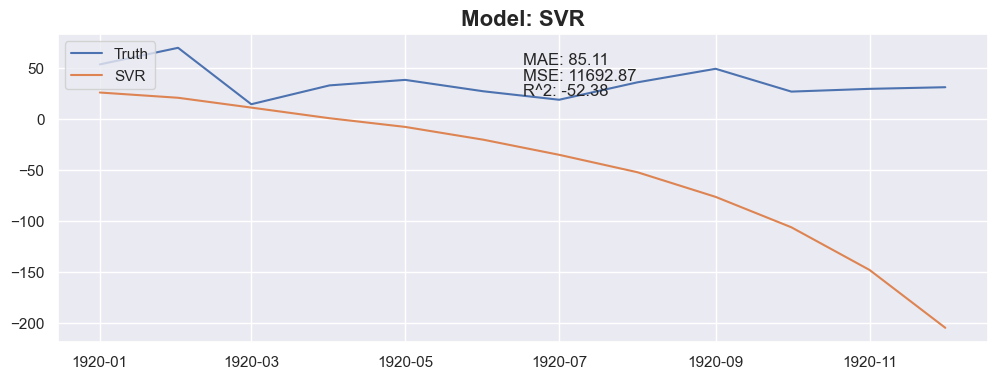
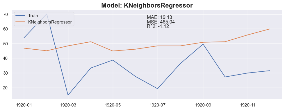
### Compare Models
```python
def predict_next(months: int, df_X_train: pd.DataFrame(), df_y_train: pd.DataFrame() , model_: sklearn.linear_model) -> pd.DataFrame():
df_y_train = pd.DataFrame(df_y_train, columns=['Sunspots'])
# I will use the last row of the train set as the first prediction input
for i in range(months):
# this value correspond to the next month
sunspot_pred = model_.predict( df_X_train.tail(1) )
# get the last date of the df_train and add one month
last_date = df_train.tail(1).index + pd.DateOffset(months=1)
# create a df, date as index and prediction as value to the prediction set
row_pred = pd.DataFrame(data=[sunspot_pred], columns=df_y_train.columns , index=last_date)
# add the prediction row at the at to the prediction set in the only column
df_y_train = pd.concat([df_y_train, row_pred])
# also, prepend the very first sunspot that has been removed with the shift
first_sunspot = df_train['Sunspots'].head(1)
first_sunspot = pd.DataFrame(first_sunspot, columns=['Sunspots'])
df_y_train = pd.concat([first_sunspot, df_y_train])
# create the new dataframe for the prediction set based on the new prediction
df_X_train = parse_df(df_y_train)
# then shift y again
df_y_train = df_y_train.shift(-1).dropna()
return df_y_train[-months:]
```
```python
import sklearn
# Models to use
models = [
LinearRegression(),
DecisionTreeRegressor(),
RandomForestRegressor(),
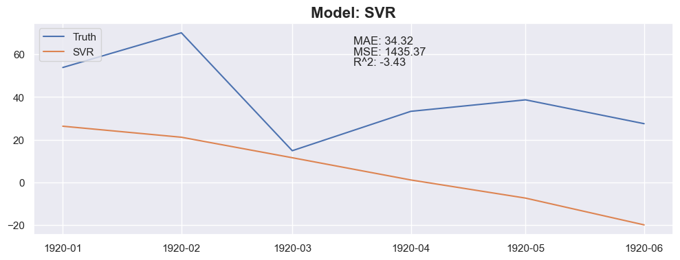
SVR(kernel='poly'), # SVM regressor
KNeighborsRegressor(),
MLPRegressor(),
]
months_to_predict_array = [3, 6, 12]
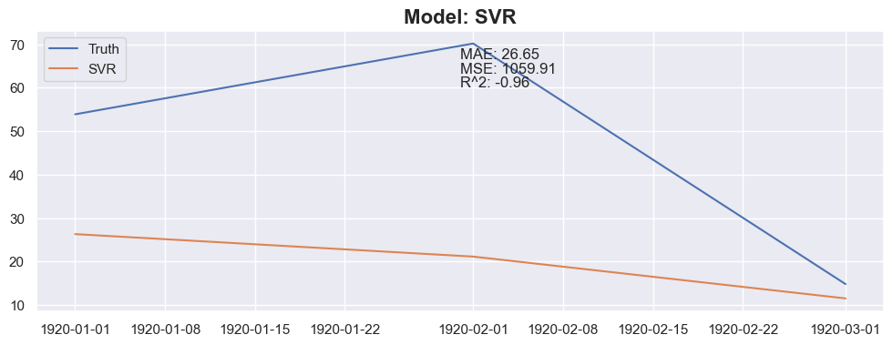
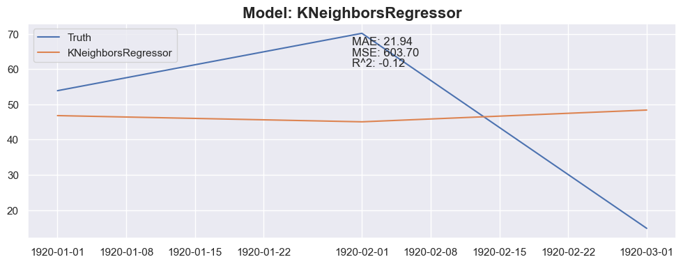
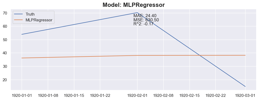
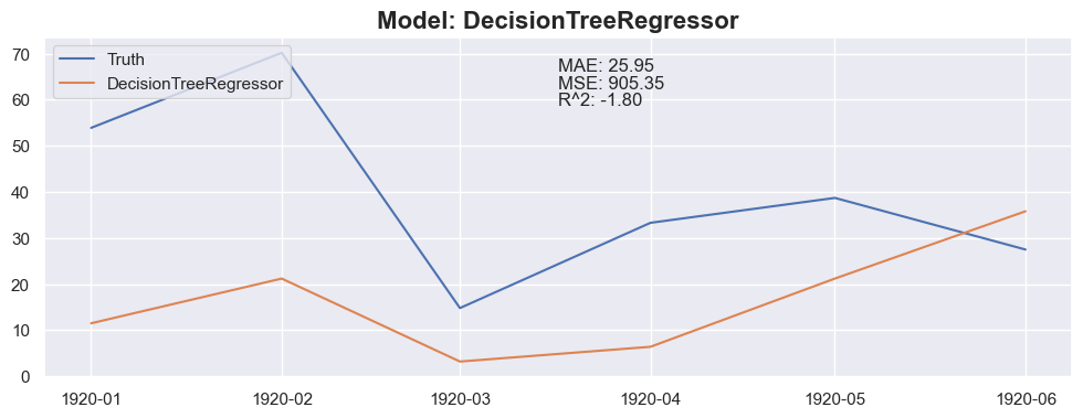
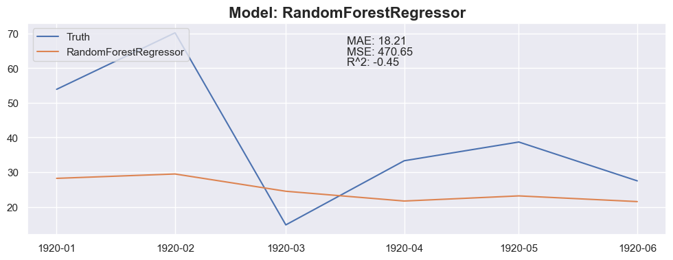
for months_to_predict in months_to_predict_array:
for model in models:
X_train_model = X_train.copy()
X_test_model = X_test.copy()
y_train_model = y_train.copy()
y_test_model = y_test.copy()
# fit the model, don't use the last row since has no truth
model = model.fit(X_train_model[:-1], y_train_model)
model_name = model.__class__.__name__
y_pred = predict_next(months_to_predict, X_train_model, y_train_model, model)
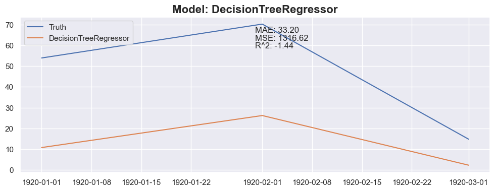
plt.figure(figsize=(12, 4))
# plt.plot(X_train_model[:-1].index, y_train_model, label='Train')
plt.plot(X_test_model[:months_to_predict].index, y_test_model[:months_to_predict], label='Truth')
plt.plot(X_test_model[:months_to_predict].index, y_pred, label=model_name)
plt.legend(loc='upper left')
mae = mean_absolute_error(y_test_model[:months_to_predict], y_pred)
mse = mean_squared_error(y_test_model[:months_to_predict], y_pred)
r2 = r2_score(y_test_model[:months_to_predict], y_pred)
plt.title(f"Model: {model_name}", fontsize=16, fontweight='bold')
plt.text(0.5, 0.9, f"MAE: {mae:.2f}", transform=plt.gca().transAxes)
plt.text(0.5, 0.85, f"MSE: {mse:.2f}", transform=plt.gca().transAxes)
plt.text(0.5, 0.8, f"R^2: {r2:.2f}", transform=plt.gca().transAxes)
```
C:\ProgramData\anaconda3\envs\MachineLearning\lib\site-packages\sklearn\neural_network\_multilayer_perceptron.py:686: ConvergenceWarning: Stochastic Optimizer: Maximum iterations (200) reached and the optimization hasn't converged yet.
warnings.warn(
C:\ProgramData\anaconda3\envs\MachineLearning\lib\site-packages\sklearn\neural_network\_multilayer_perceptron.py:686: ConvergenceWarning: Stochastic Optimizer: Maximum iterations (200) reached and the optimization hasn't converged yet.
warnings.warn(
C:\ProgramData\anaconda3\envs\MachineLearning\lib\site-packages\sklearn\neural_network\_multilayer_perceptron.py:686: ConvergenceWarning: Stochastic Optimizer: Maximum iterations (200) reached and the optimization hasn't converged yet.
warnings.warn(
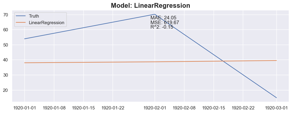
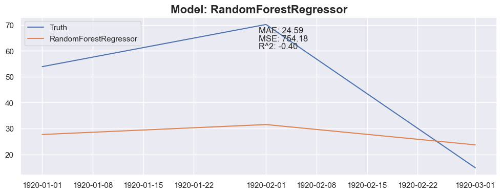
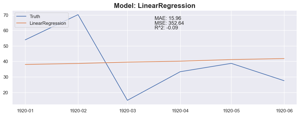
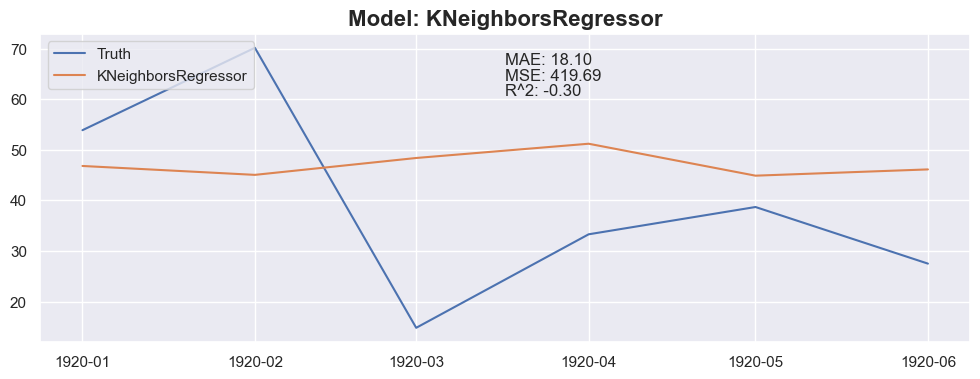
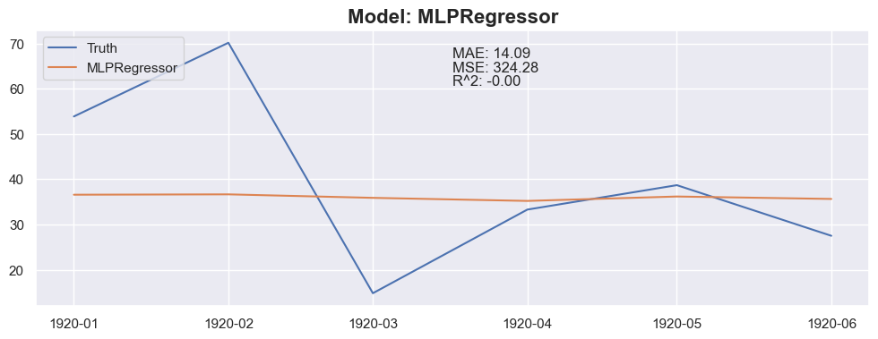
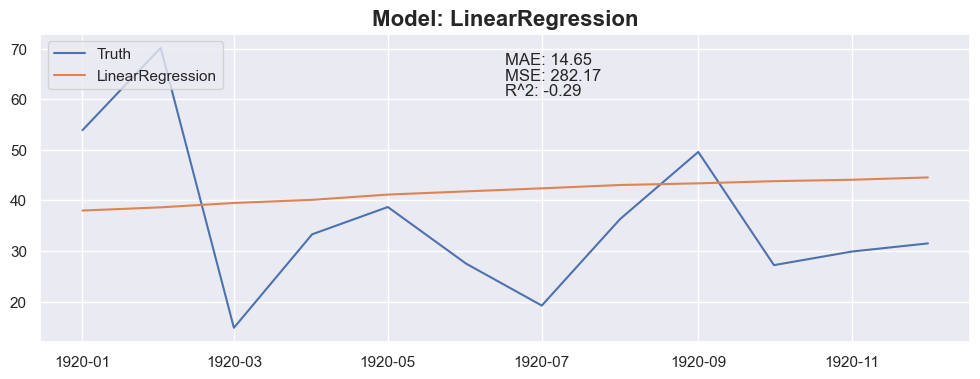
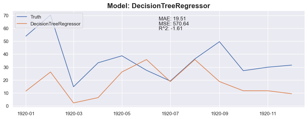
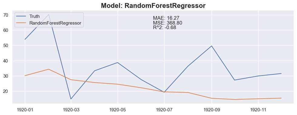
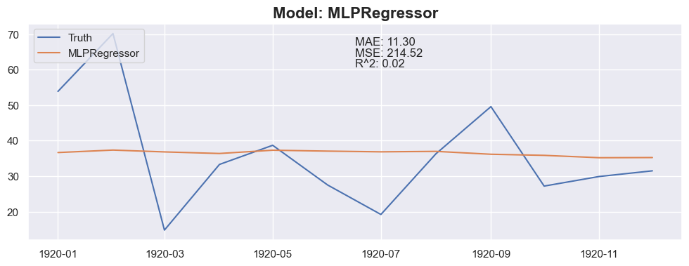
### Conclusion
The linear regression with default value has a perfect score, so I think I could be happy with this result and stop here.
# Optional : Darts
Tring using the [Darts library](https://unit8.com/resources/darts-time-series-made-easy-in-python/).
```python
from darts import TimeSeries
```
```python
df_darts = pd.read_csv('data/monthly-sunspots.csv')
df_darts.head()
```
|
Month |
Sunspots |
| 0 |
1749-01 |
58.0 |
| 1 |
1749-02 |
62.6 |
| 2 |
1749-03 |
70.0 |
| 3 |
1749-04 |
55.7 |
| 4 |
1749-05 |
85.0 |
```python
series = TimeSeries.from_dataframe(df_darts, 'Month', 'Sunspots')
series.plot()
```
```python
from darts.dataprocessing.transformers import Scaler
scaler = Scaler()
series_scaled = scaler.fit_transform(series)
series_scaled.plot()
```

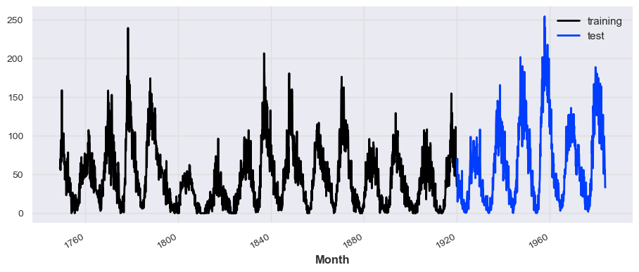
## Splitting the series
```python
train_series, test_series = series.split_before(pd.Timestamp('19200101'))
train_series.plot(label='training')
test_series.plot(label='test')
```
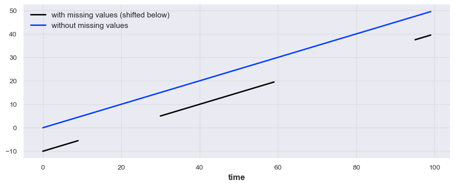
## Missing values
```python
# example code
from darts.utils.missing_values import fill_missing_values
values = np.arange(50, step=0.5)
values[10:30] = np.nan
values[60:95] = np.nan
series_ = TimeSeries.from_values(values)
(series_ - 10).plot(label="with missing values (shifted below)")
fill_missing_values(series_).plot(label="without missing values")
```
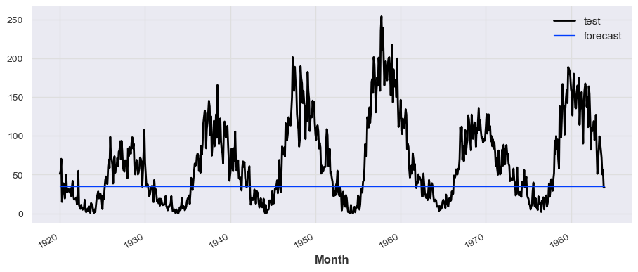
## Train and predict
```python
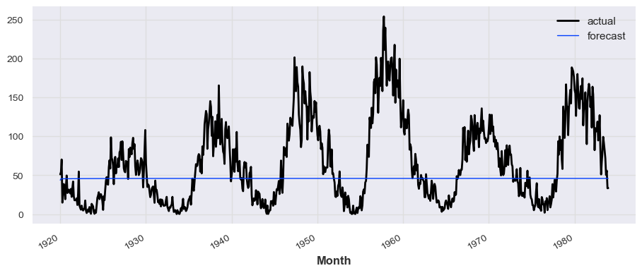
from darts.models import NaiveSeasonal
model = NaiveSeasonal(K=1)
model.fit(train_series)
prediction = model.predict(len(test_series))
# train_series.plot(label='actual')
test_series.plot(label='test')
prediction.plot(label='forecast', lw=1)
plt.legend()
```
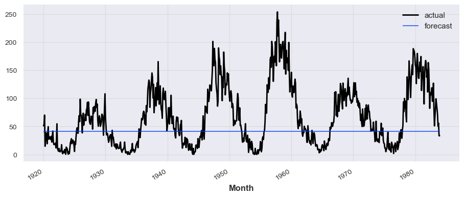
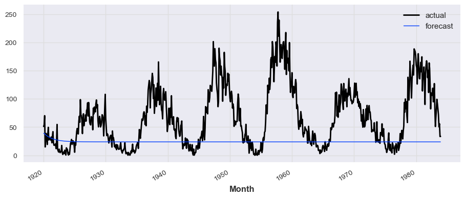
```python
from darts.models import ExponentialSmoothing
model = ExponentialSmoothing()
model.fit(train_series)
prediction_exp = model.predict(len(test_series))
# train_series.plot(label='actual')
test_series.plot(label='actual')
prediction_exp.plot(label='forecast', lw=1)
plt.legend()
```
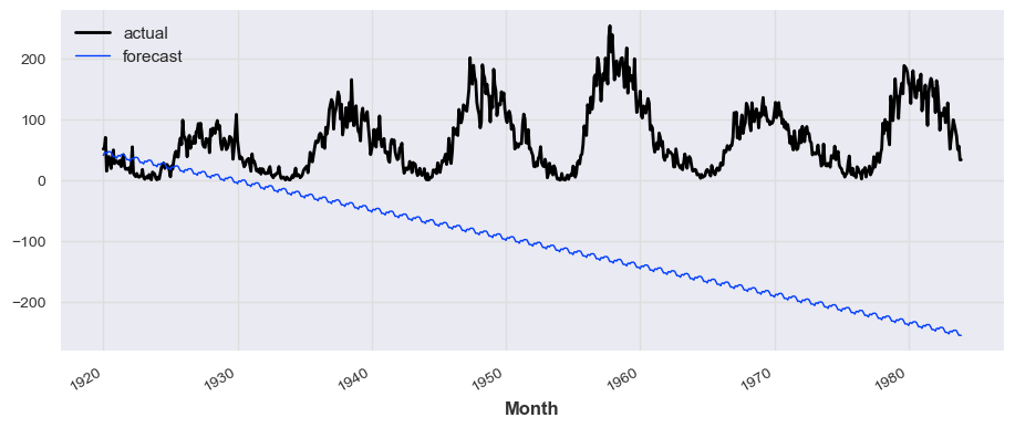
```python
from darts.models import AutoARIMA
model_aarima = AutoARIMA()
model_aarima.fit(train_series)
prediction_aarima = model_aarima.predict(len(test_series))
# train_series.plot(label='actual')
test_series.plot(label='actual')
prediction_aarima.plot(label='forecast', lw=1)
plt.legend()
```
```python
from darts.models import Prophet
model_prophet = Prophet()
model_prophet.fit(train_series)
prediction_prophet = model_prophet.predict(len(test_series))
# train_series.plot(label='actual')
test_series.plot(label='actual')
prediction_prophet.plot(label='forecast', lw=1)
plt.legend()
```
08:29:59 - cmdstanpy - INFO - Chain [1] start processing
08:29:59 - cmdstanpy - INFO - Chain [1] done processing
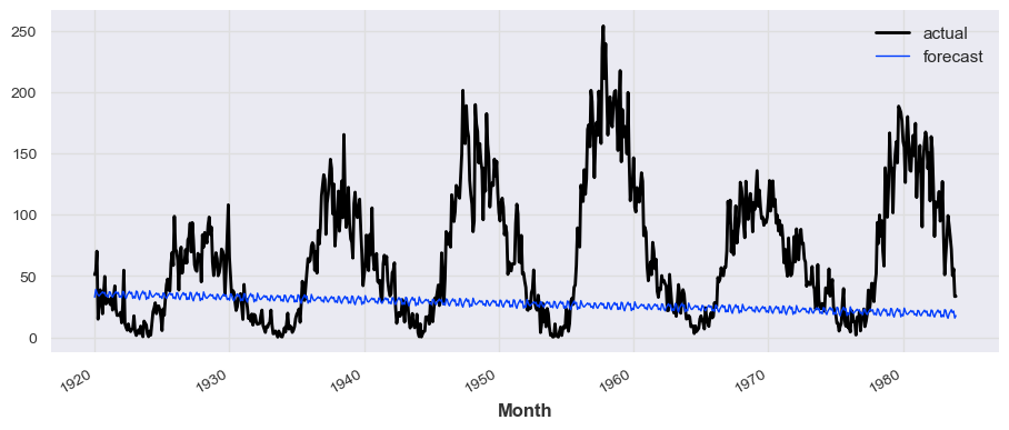
```python
from darts.models import RNNModel, TCNModel, TransformerModel
model_rnn = RNNModel( input_chunk_length=12, output_chunk_length=1, n_epochs=30, model_name='LSTM')
model_rnn.fit(train_series, verbose=True)
prediction_rnn = model_rnn.predict(len(test_series))
# train_series.plot(label='actual')
test_series.plot(label='actual')
prediction_rnn.plot(label='forecast', lw=1)
plt.legend()
```
ignoring user defined `output_chunk_length`. RNNModel uses a fixed `output_chunk_length=1`.
GPU available: False, used: False
TPU available: False, using: 0 TPU cores
IPU available: False, using: 0 IPUs
HPU available: False, using: 0 HPUs
| Name | Type | Params
---------------------------------------------------
0 | criterion | MSELoss | 0
1 | train_metrics | MetricCollection | 0
2 | val_metrics | MetricCollection | 0
3 | rnn | RNN | 700
4 | V | Linear | 26
---------------------------------------------------
726 Trainable params
0 Non-trainable params
726 Total params
0.003 Total estimated model params size (MB)
Training: 0it [00:00, ?it/s]
`Trainer.fit` stopped: `max_epochs=30` reached.
GPU available: False, used: False
TPU available: False, using: 0 TPU cores
IPU available: False, using: 0 IPUs
HPU available: False, using: 0 HPUs
Predicting: 0it [00:00, ?it/s]
```python
model_tcn = TCNModel(input_chunk_length=12, output_chunk_length=1, n_epochs=30)
model_tcn.fit(train_series, verbose=True)
prediction_tcn = model_tcn.predict(len(test_series))
# train_series.plot(label='actual')
test_series.plot(label='actual')
prediction_tcn.plot(label='forecast', lw=1)
plt.legend()
```
GPU available: False, used: False
TPU available: False, using: 0 TPU cores
IPU available: False, using: 0 IPUs
HPU available: False, using: 0 HPUs
| Name | Type | Params
----------------------------------------------------
0 | criterion | MSELoss | 0
1 | train_metrics | MetricCollection | 0
2 | val_metrics | MetricCollection | 0
3 | dropout | MonteCarloDropout | 0
4 | res_blocks | ModuleList | 92
----------------------------------------------------
92 Trainable params
0 Non-trainable params
92 Total params
0.000 Total estimated model params size (MB)
Training: 0it [00:00, ?it/s]
`Trainer.fit` stopped: `max_epochs=30` reached.
GPU available: False, used: False
TPU available: False, using: 0 TPU cores
IPU available: False, using: 0 IPUs
HPU available: False, using: 0 HPUs
Predicting: 0it [00:00, ?it/s]
```python
model_transformer = TransformerModel(input_chunk_length=12, output_chunk_length=1, n_epochs=30)
model_transformer.fit(train_series, verbose=True)
prediction_transformer = model_transformer.predict(len(test_series))
# train_series.plot(label='actual')
test_series.plot(label='actual')
prediction_transformer.plot(label='forecast', lw=1)
plt.legend()
```
GPU available: False, used: False
TPU available: False, using: 0 TPU cores
IPU available: False, using: 0 IPUs
HPU available: False, using: 0 HPUs
| Name | Type | Params
------------------------------------------------------------
0 | criterion | MSELoss | 0
1 | train_metrics | MetricCollection | 0
2 | val_metrics | MetricCollection | 0
3 | encoder | Linear | 128
4 | positional_encoding | _PositionalEncoding | 0
5 | transformer | Transformer | 548 K
6 | decoder | Linear | 65
------------------------------------------------------------
548 K Trainable params
0 Non-trainable params
548 K Total params
2.195 Total estimated model params size (MB)
Training: 0it [00:00, ?it/s]
`Trainer.fit` stopped: `max_epochs=30` reached.
GPU available: False, used: False
TPU available: False, using: 0 TPU cores
IPU available: False, using: 0 IPUs
HPU available: False, using: 0 HPUs
Predicting: 0it [00:00, ?it/s]

## Evaluation
```python
from darts.metrics import mape, mase
print('Prophet')
print('MAPE: {:.2f}%'.format(mape(prediction_prophet, test_series)))
print('MASE: {:.2f}'.format(mase(prediction_prophet, test_series, train_series)))
print('R^2: {:.2f}'.format(r2_score(test_series.values(), prediction_prophet.values())))
print('AutoARIMA')
print('MAPE: {:.2f}%'.format(mape(prediction_aarima, test_series)))
print('MASE: {:.2f}'.format(mase(prediction_aarima, test_series, train_series)))
print('R^2: {:.2f}'.format(r2_score(test_series.values(), prediction_aarima.values())))
print('Exponential Smoothing')
print('MAPE: {:.2f}%'.format(mape(prediction_exp, test_series)))
print('MASE: {:.2f}'.format(mase(prediction_exp, test_series, train_series)))
print('R^2: {:.2f}'.format(r2_score(test_series.values(), prediction_exp.values())))
print('RNN')
print('MAPE: {:.2f}%'.format(mape(prediction_rnn, test_series)))
print('MASE: {:.2f}'.format(mase(prediction_rnn, test_series, train_series)))
print('R^2: {:.2f}'.format(r2_score(test_series.values(), prediction_rnn.values())))
print('TCN')
print('MAPE: {:.2f}%'.format(mape(prediction_tcn, test_series)))
print('MASE: {:.2f}'.format(mase(prediction_tcn, test_series, train_series)))
print('R^2: {:.2f}'.format(r2_score(test_series.values(), prediction_tcn.values())))
print('Transformer')
print('MAPE: {:.2f}%'.format(mape(prediction_transformer, test_series)))
print('MASE: {:.2f}'.format(mase(prediction_transformer, test_series, train_series)))
print('R^2: {:.2f}'.format(r2_score(test_series.values(), prediction_transformer.values())))
```
Prophet
MAPE: 195.49%
MASE: 4.25
R^2: -0.62
AutoARIMA
MAPE: 94.51%
MASE: 3.76
R^2: -0.16
Exponential Smoothing
MAPE: 558.50%
MASE: 15.00
R^2: -14.13
RNN
MAPE: 106.90%
MASE: 3.83
R^2: -0.23
TCN
MAPE: 207.13%
MASE: 4.29
R^2: -0.67
Transformer
MAPE: 94.76%
MASE: 3.77
R^2: -0.16